Structure functions#

This documentation page lists all $F_{2 / L} (x_{B j}, Q^{2})$ nucleon structure functions types modelled and embedded in the CepGen library. These modellings are intensively used in the photon fluxes computation, and each of these are tuned for a specific kinematics range.

All parameterisations derive from the following base class:

class Parameterisation : public NamedModule<Parameterisation>#: Subclassed by PartonicParameterisation

Detailed description

Click to show

class Parameterisation : public NamedModule<Parameterisation>

Base object for the parameterisation of nucleon structure functions.

Subclassed by PartonicParameterisation

Public Functions

inline virtual bool hasW1W2() const: provides modelling for W_1/W_2? Longitudinal/transverse cross section ratio parameterisation used to compute $F_{1 / L}$

Parameterisation &operator()(double xbj, double q2)

Compute all relevant structure functions for a given $(x_{B j}, Q^{2})$ couple.

Parameters:

xbj – [in] Bjorken’s x variable
q2 – [in] Squared 4-momentum transfer (in GeV^2)

double F2(double xbj, double q2): Transverse structure function.

double FL(double xbj, double q2): Longitudinal structure function.

double W1(double xbj, double q2): Longitudinal form factor.

double FE(double xbj, double q2): Electric proton form factor.

double FM(double xbj, double q2): Magnetic proton form factor.

double F1(double xbj, double q2): $F_{1}$ structure function

inline const std::string &name() const: Module unique indexing name.

inline bool operator==(const SteeredObject &oth) const: Equality operator.

inline bool operator!=(const SteeredObject &oth) const: Inequality operator.

inline virtual const ParametersList &parameters() const override: Module user-defined parameters.

inline virtual void setParameters(const ParametersList &params) override: Set module parameters.

inline void setDescribedParameters(const ParametersList &params_orig): Set (documented) module parameters.

Public Static Functions

static ParametersDescription description(): Generic description for the structure functions.

Friends

friend std::ostream &operator<<(std::ostream&, const Parameterisation&): Human-readable dump of the SF parameterisation at this (xBj,Q^2) value.

struct Arguments

struct Values

Public Members

double f2 = {0.}: Last computed transverse structure function value.

double fl = {0.}: Last computed longitudinal structure function value.

double w1 = {0.}: Longitudinal form factor.

double fe = {0.}: Electric proton form factor.

double fm = {0.}: Magnetic proton form factor.

Note

All of these may be used and linked against any external code.

The parameterisation types handled in CepGen are listed in the cepgen::StructureFunctionsFactory.

Below, a semi-detailed review of a subset of the modellings handled in CepGen is presented.

Whenever not specified explicitely in the modelling, the $F_{L}$ structure function can be computed from the $R$ modelling-dependent relation:

F_{L} (x_{B j}, Q^{2}) = (1 + \frac{4 m_{p}^{2} {x_{B j}}^{2}}{Q^{2}}) \frac{R}{1 + R} F_{2} (x_{B j}, Q^{2}) .

Where this $R$ ratio can be evaluated for any $(x_{B j}, Q^{2})$ range of interest .

Hybrid models#

As the name suggests, this class of model combines multiple extrapolation models valid in multiple kinematic ranges into a set of uniform, continuous structure functions.

Shamov#

Note

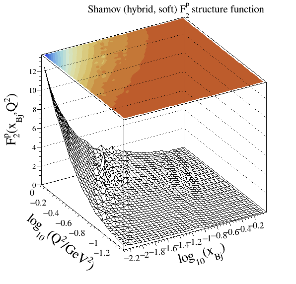
Legacy code: 302
Structure functions modelled: $W_{1}$ , $W_{2}$ , $F_{2}$
Implementation: cepgen::strfun::Shamov
Module parameters

This model is designed for soft, low- $Q^{2}$ regimes under a broad range of $x_{B j}$ . Several operation modes are proposed, steered by the mode parameter:

SuriYennie, the standard, Suri and Yennie continuum (see below) ;
RealRes, using a linear grid interpolation of the real photon cross section for $Q^{2} \to 0$ with resonances dependance as for $Δ (1232)$ ;
RealResAndNonRes, like the earlier, and using the Suri and Yennie non-resonant contribution ;
RealAndSuriYennieNonRes, using the Suri and Yennie non-resonant contribution ;
RealAndFitNonRes, like the RealResAndNonRes, but using a fit for the non-resonant contributions.

Kulagin-Barinov#

Note

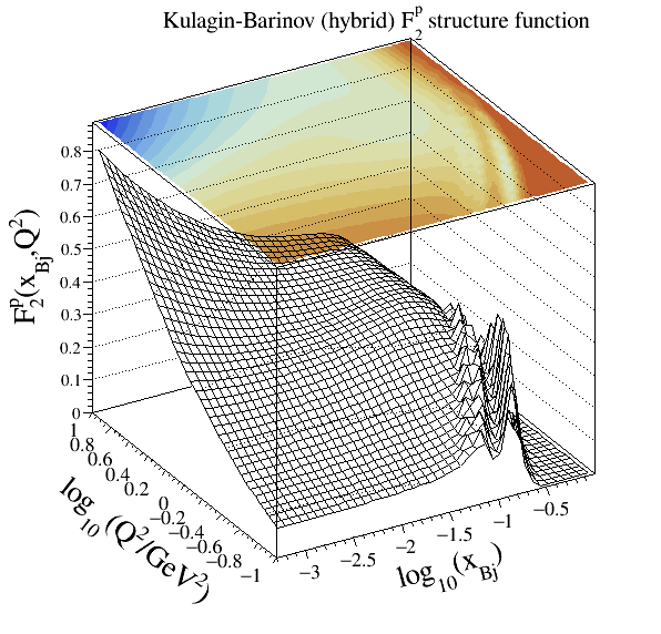
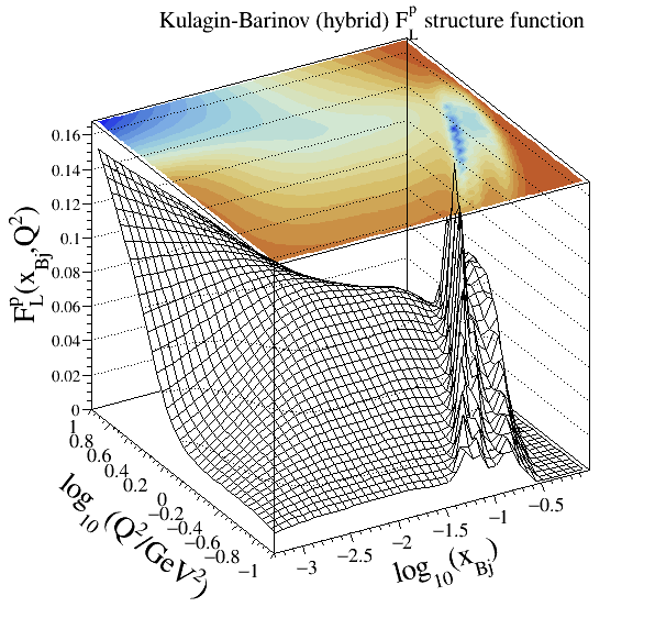
Legacy code: 303
Structure functions modelled: $F_{2}$ , $F_{L}$
Reference:
Implementation: cepgen::strfun::KulaginBarinov
Module parameters

Resonances are modelled through Breit-Wigner contributions from five states. For the DIS part, a higher twist correction is available from a global QCD fit.

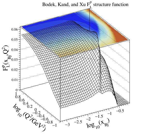
Bodek-Kang-Xu#

Note

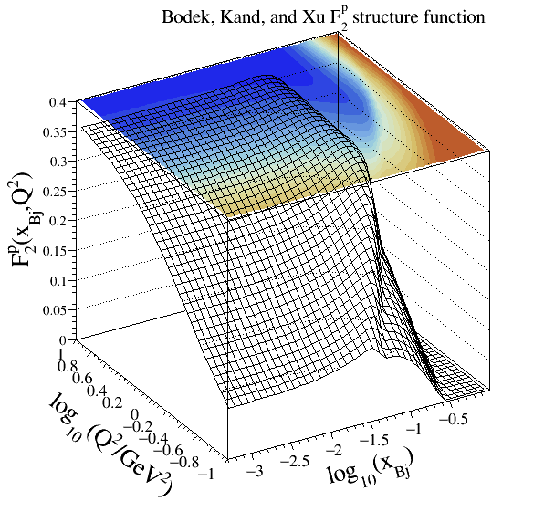
Legacy code: 304
Structure functions modelled: $F_{1}$ , $F_{2}$
Reference:
Implementation: cepgen::strfun::BodekKangXu
Module parameters

Continuum models#

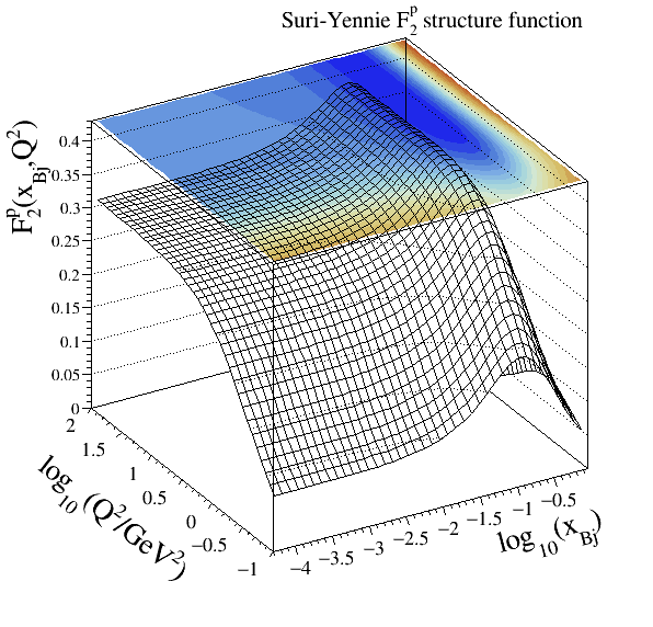
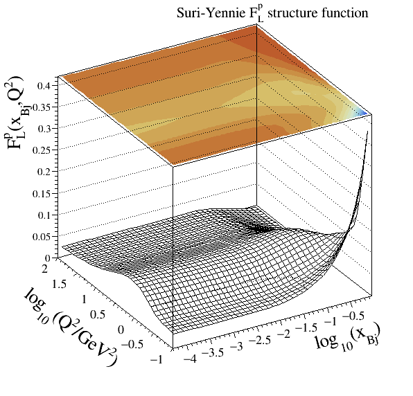
Suri-Yennie#

Note

Legacy code: 11 (and 12 for the alternative parameterisation)
Structure functions modelled: $F_{E}$ , $F_{M}$
Reference:
Implementations: cepgen::strfun::SuriYennie and cepgen::strfun::SuriYennieAlt
Module parameters: main and alternative parameterisations

This set was used as a standard option in the LPAIR event generator. It provides a reasonable description of SLAC data in the resonance and continuum regions.

Szczurek-Uleshchenko#

Note

Legacy code: 12
Structure function modelled: $F_{2}$
Reference:
Implementation: cepgen::strfun::SzczurekUleshchenko, relying on the GRV Fortran interpolation subroutine
Module parameters

This set puts an emphasis on the low-to-intermediate $Q^{2}$ region and includes a smooth continuation to low- $Q^{2}$ .

Block-Durand-Ha#

Note

Legacy code: 13
Structure function modelled: $F_{2}$
Reference:
Implementation: cepgen::strfun::BlockDurandHa
Module parameters

ALLM parameterisation#

Note

Structure function modelled: $F_{2}$
References:

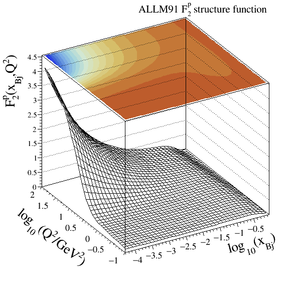
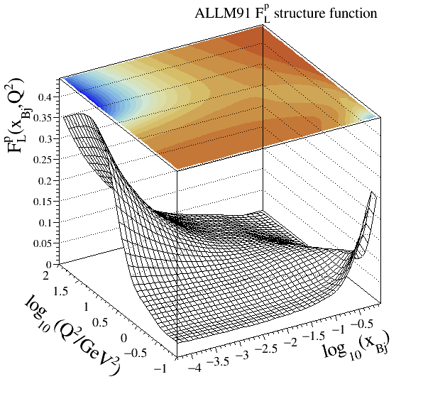
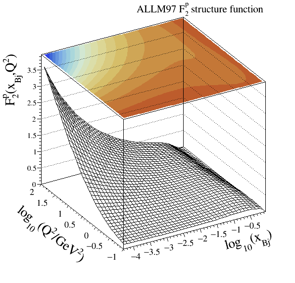
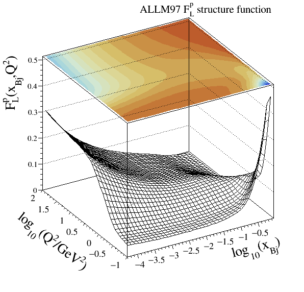
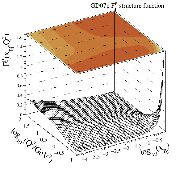
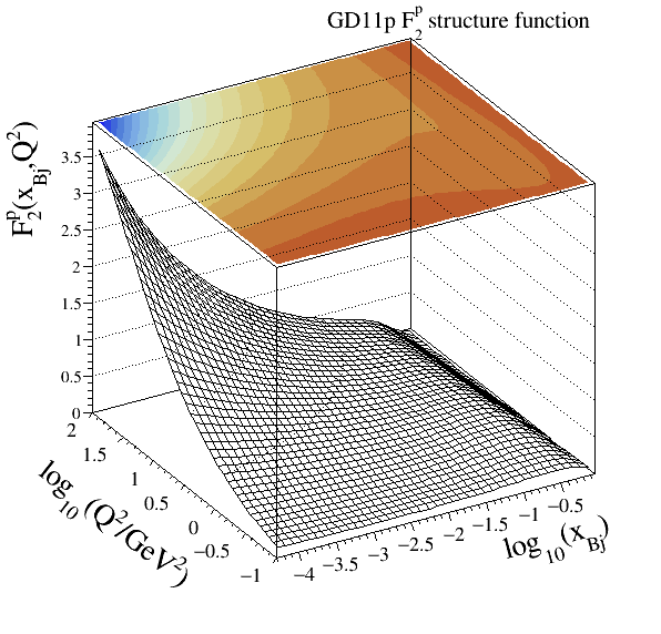
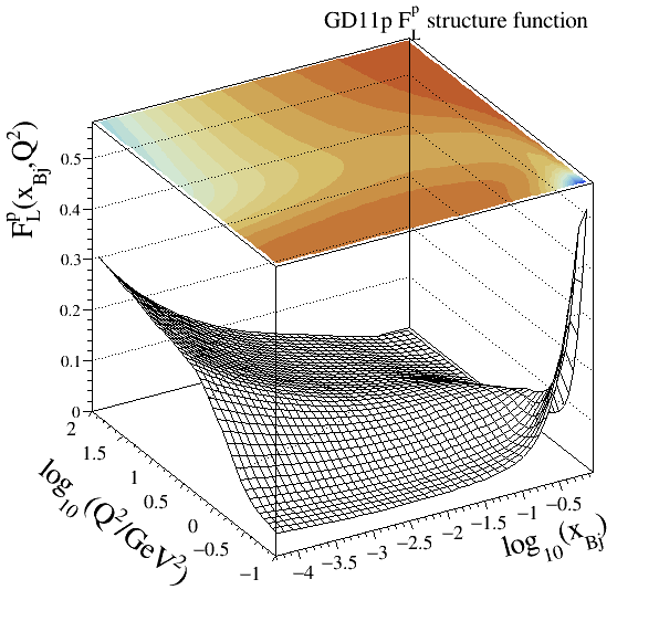
A full reference of this parameterisation by Abramowicz et al. can be found in (ALLM91) and (ALLM97). The HERMES Collaboration refits of this modelling, labelled GD07p and GD11p may be found in .
Parameterisations:
- ALLM91
  - Legacy code: 201
  - Implementation: cepgen::strfun::ALLM91
  - Module parameters
- ALLM97
  - Legacy code: 202
  - Implementation: cepgen::strfun::ALLM97
  - Module parameters
- GD07p
  - Legacy code: 203
  - Implementation: cepgen::strfun::GD07p
  - Module parameters
- GD11p
  - Legacy code: 204
  - Implementation: cepgen::strfun::GD11p
  - Module parameters
- HHTALLM
  - Legacy code: 206
  - Implementation: cepgen::strfun::HHTALLM
  - Module parameters
- HHTALLMFT
  - Legacy code: 207
  - Implementation: cepgen::strfun::HHTALLMFT
  - Module parameters

In this continuum region modelling the $F_{2}$ proton structure function is parameterised as:

F_{2} (x_{B j}, Q^{2}) = \frac{Q^{2}}{Q^{2} + m_{0}^{2}} [F_{2}^{I P} (x_{B j}, Q^{2}) + F_{2}^{I R} (x_{B j}, Q^{2})],

with $m_{0}$ the effective photon mass. The pomeron/reggeon exchanges terms are parameterised as:

F_{2}^{I P, I R} (x_{B j}, Q^{2}) = c^{I P, I R} (t) x_{I P, I R}^{a^{I P, I R} (t)} (1 - x_{B j})^{b^{I P, I R} (t)},

with the slowly-varying function $t = t (Q^{2})$ defined as:

t (Q^{2}) = \ln (\ln \frac{Q^{2} + Q_{0}^{2}}{Λ^{2}}) - \ln (\ln \frac{Q_{0}^{2}}{Λ^{2}}),

and the modified Bjorken- $x$ functions:

x_{I P, I R} = {(1 + \frac{w^{2} - m_{p}^{2}}{Q^{2} + m_{I P, I R}})}^{- 1} .

The six functionals $a^{I P, I R} (t), b^{I P, I R} (t), c^{I P, I R} (t)$ are parameterised as:

\begin{array}{r} a^{I P} (t) = a_{1}^{I P} + (a_{1}^{I P} - a_{2}^{I P}) [\frac{1}{1 + t^{a_{3}^{I P}}} - 1], \\ b^{I P} (t) = b_{1}^{I P} + b_{2}^{I P} t^{b_{3}^{I P}}, \\ c^{I P} (t) = c_{1}^{I P} + (c_{1}^{I P} - c_{2}^{I P}) [\frac{1}{1 + t^{c_{3}^{I P}}} - 1] \end{array}

for the pomeron part, and

\begin{array}{r} a^{I R} (t) = a_{1}^{I R} + a_{2}^{I R} t^{a_{3}^{I R}}, \\ b^{I R} (t) = b_{1}^{I R} + b_{2}^{I R} t^{b_{3}^{I R}}, \\ c^{I R} (t) = c_{1}^{I R} + c_{2}^{I R} t^{c_{3}^{I R}}, \end{array}

for the reggeon subset.

Currently, four tunings of the 23 model parameters are embedded within CepGen:

Parameter	Units	ALLM91	ALLM97	GD07p	GD11p
$m_{0}^{2}$	GeV $^{2}$	0.30508	0.31985	0.454	0.5063
$m_{I P}^{2}$	GeV $^{2}$	10.676	49.457	30.7	34.75
$m_{I R}^{2}$	GeV $^{2}$	0.20623	0.15052	0.117	0.03190
$Q_{0}^{2}$	GeV $^{2}$	0.27799	0.52544	1.15	1.374
$Λ_{0}^{2}$	GeV $^{2}$	0.06527	0.06527	0.06527	0.06527
$a_{1}^{I P}$	-	-0.04503	-0.0808	-0.105	-0.11895
$a_{2}^{I P}$	-	-0.36407	-0.44812	-0.495	-0.4783
$a_{3}^{I P}$	-	8.17091	1.1709	1.29	1.353
$b_{1}^{I P}$	-	0.49222	0.36292	-1.42	1.0833
$b_{2}^{I P}$	-	0.52116	1.8917	4.51	2.656
$b_{3}^{I P}$	-	3.5515	1.8439	0.551	1.771
$c_{1}^{I P}$	-	0.26550	0.28067	0.339	0.3638
$c_{2}^{I P}$	-	0.04856	0.22291	0.127	0.1211
$c_{3}^{I P}$	-	1.04682	2.1979	1.16	1.166
$a_{1}^{I R}$	-	0.60408	0.584	0.374	0.3425
$a_{2}^{I R}$	-	0.17353	0.37888	0.998	1.0603
$a_{3}^{I R}$	-	1.61812	2.6063	0.775	0.5164
$b_{1}^{I R}$	-	1.26066	0.01147	2.71	-10.408
$b_{2}^{I R}$	-	1.83624	3.7582	1.83	14.857
$b_{3}^{I R}$	-	0.81141	0.49338	1.26	0.07739
$c_{1}^{I R}$	-	0.67639	0.80107	0.838	1.3633
$c_{2}^{I R}$	-	0.49027	0.97307	2.36	2.256
$c_{3}^{I R}$	-	2.66275	3.4942	1.77	2.209

The ALLM91 tuning is fitted from all pre-HERA data points available.

Resonance models#

Fiore-Brasse#

Note

Legacy code: 101 (core), and 104 (alternative)
Structure function modelled: $F_{2}$
References:
Implementation: cepgen::strfun::FioreBrasse, and cepgen::strfun::FioreBrasseAlt
Modules parameters: core and alternative parameterisations

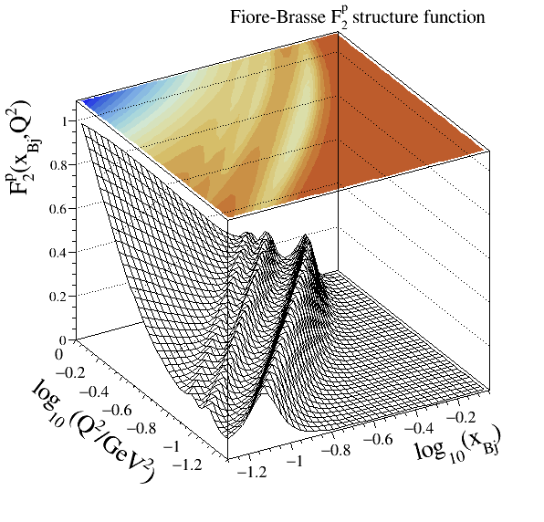
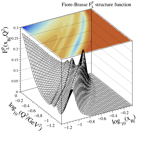
This parameterisation gives a very good description of photoabsorption in the resonance region from low to large $Q^{2}$ . It is designed to reproduce well JLAB and SLAC data.

Christy-Bosted#

Note

Legacy code: 102
Structure functions modelled: $F_{2}$ , $F_{L}$
Reference:
Implementation: cepgen::strfun::ChristyBosted
Module parameters

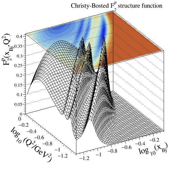
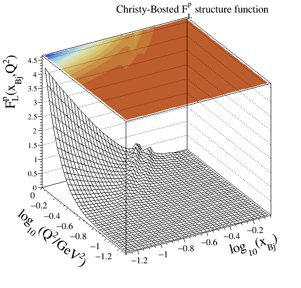
The set developed by M.E. Christy and P.E. Bosted is emphasised on the very-low $Q^{2}$ regime, with its particular use of JLAB’s Hall-C data on:

inclusive inelastic (up to $Q^{2} s i m e q$ 7.5 GeV²),
photoproduction at $Q^{2}$ = 0, and
DIS data at high- $(Q^{2}, W)$ .

CLAS#

Note

Legacy code: 103
Structure functions modelled: $F_{2}$
Reference:
Implementation: cepgen::strfun::CLAS
Module parameters

Perturbative models#

MSTW grid#

Warning

doxygenclass: Cannot find class “mstw::Grid” in doxygen xml output for project “CepGen” from directory: /Documentation/build/xml

External interfaces#

Several other models can also be interfaced through a base partonic structure functions interface allowing the conversion of PDFs into $F_{2}$ / $F_{L}$ structure functions. This object has the form:

class PartonicParameterisation : public Parameterisation #

The conversion of quark/gluon PDF content into $F_{2}$ structure function is computed as follows:

\begin{array}{r} F_{2}^{v a l} (x_{B j}, Q^{2}) = \sum_{i = 1}^{n_{q}} e_{i}^{2} [q_{i} (x_{B j}, Q^{2}) - {\bar{q}}_{i} (x_{B j}, Q^{2})] \\ F_{2}^{s e a} (x_{B j}, Q^{2}) = 2 \sum_{i = 1}^{n_{q}} e_{i}^{2} {\bar{q}}_{i} (x_{B j}, Q^{2}) \\ F_{2}^{t o t} (x_{B j}, Q^{2}) = F_{2}^{v a l} (x_{B j}, Q^{2}) + F_{2}^{s e a} (x_{B j}, Q^{2}) \end{array}

LHAPDF interface#

Note

Legacy code: 401 (“standard” parameterisation), or a more complex scheme: : The legacy-equivalent signature follows the convention 1MSSSSSS, where:
- M specifies the set of partons included in the sum rule: : - 0: all partons,
  - 1: valence quarks only, and
  - 2: sea quarks only.
- SSSSSS is the integer LHAPDF ID code for the selected PDF set.
Structure function modelled: $F_{2}$
Reference:
Implementation: cepgen::strfun::LHAPDFPartonic
Module parameters

APFEL++ interface#

Note

Legacy code: 405
Structure function modelled: $F_{2}$ , $F_{L}$
Reference:
Implementation: cepgen::apfelpp::EvolutionStructureFunctions
Module parameters

This interface to the APFEL++ C++ rewriting of the famous APFEL library covers the computation of order-0/1/2/3 perturbative $F_{2, L}$ under several assumptions/modellings. In particular, two DIS processes are currently handled for the building of interpolation grids: charged currents and neutral currents.

Structure functions

Contents

Structure functions#

Hybrid models#

Shamov#

Kulagin-Barinov#

Bodek-Kang-Xu#

Continuum models#

Suri-Yennie#

Szczurek-Uleshchenko#

Block-Durand-Ha#

ALLM parameterisation#

Resonance models#

Fiore-Brasse#

Christy-Bosted#

CLAS#

Perturbative models#

MSTW grid#

External interfaces#

LHAPDF interface#

APFEL++ interface#